Dashboard overview
Header
Use the menu to select a species or pathogen group to display. Each pathogen has its own dashboard configuration that is customised to show genotypes, resistances and other relevant parameters. Numbers indicate the total number of genomes and genotypes currently available in the selected dashboard.

Map
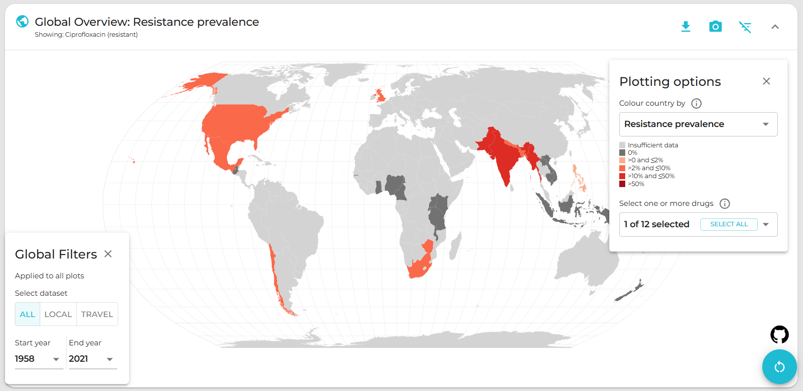
Use the Plotting options panel on the right to select a variable to display per-country summary data on the world map. Prevalence data are pooled weighted estimates of proportion for the selected resistance or genotype. A country must have N≥20 samples (using the current filters) for summary data to be displayed otherwise, it will be coloured grey to indicate insufficient data are available.
Use the Global Filter panel on the left to recalculate summary data for a specific time period and/or subgroup/s (options available vary by pathogen). Filters set in the Global Filter panel apply not only to the map, but to all plots on the page.
Clicking on a country in the map also functions as a filter, so that the Summary plots in the panels below reflect data for the selected country only. Per-country values displayed in the map can be downloaded by clicking the downward-arrow button at the top right of the panel.
Plot-specific downloads: The summary statistics currently displayed in the plot (e.g. resistance prevalence per country; with numerator, denominator and percentage) can be downloaded in tabular (TSV) format by clicking the down arrow (top-right of panel). A static image (PNG format) of the current map view can be downloaded by clicking the camera icon.
Summary plots
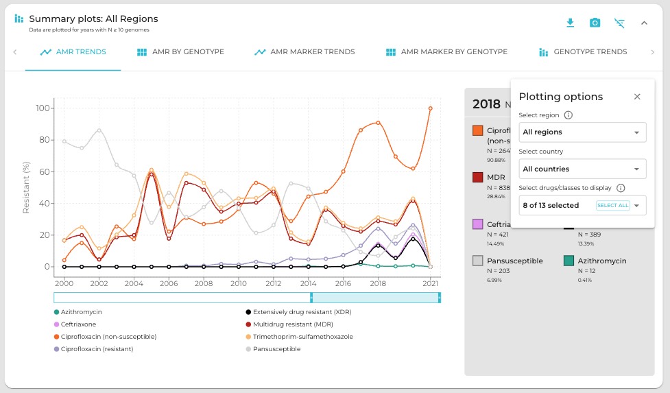
This panel offers a series of summary plots. The default view is “AMR trends”. Click a plot title in the rotating selector at the top of the panel, to choose a different plot. The specific plots available vary by pathogen, as do the definitions of AMR and genotype variables (see individual pathogen details). Summary plots are intended to show region- or country-level summaries, but if no country is selected they will populate with pooled estimates of proportion across all data passing the current filters.
All plots are interactive. Use the Plotting options panel on the right to modify the region/country to display, or to select other options available for the current plot such as which variables to display, and whether to show counts or percentages.
Line and bar plot have a dynamic legend to the right; click on an x-axis value to display counts and percentages of secondary variables calculated amongst genomes matching that x-axis value. For example, all pathogens have an ‘AMR by genotype’ plot; click a genotype to display counts and percentages of resistance estimated for each drug or class.
Plot-specific downloads: Summarised values displayed in the current plot can be downloaded by clicking the down arrow button (top-right of panel). A static image (PNG format) of the current plotting view can be downloaded by clicking the camera icon.
Geographic comparisons
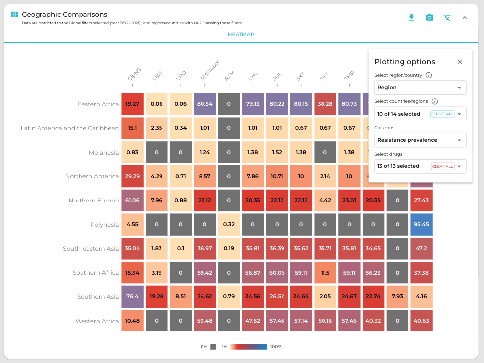
This panel uses heatmaps to explore how the prevalence of AMR or genotypes varies between countries or regions. The default view is AMR prevalence per country.
Use the Plotting options panel on the right to stratify rows by region rather than country, to view genotype prevalence instead of AMR (in columns). For some organisms, there is also the option to plot columns as resistance markers (for a selected drug).
Plotting options can also be modified to restrict the view to selected countries or regions (in rows), or to specific subsets of genotypes or drugs (in columns). Countries are not plotted (and not available to select) if the number of samples passing the current global filter is below 20. By default, the 20 most common genotypes or drugs (passing current filters) will be included in the plot; in the drop-down list to modify the specific set of drugs or genotypes shown, the available options will be ordered by their frequency in the current selection.
Plot-specific downloads: Summarised values displayed in the current heatmap can be downloaded by clicking the down arrow button (top-right of panel). A static image (PNG format) of the current plotting view can be downloaded by clicking the camera icon.
Downloads
At the bottom are buttons to download (1) the individual genome-level information that is used to populate the dashboard (‘Download database (TSV format)’); and (2) a static report of the currently displayed plots, together with a basic description of the data sources and variable definitions (‘Report view’).
